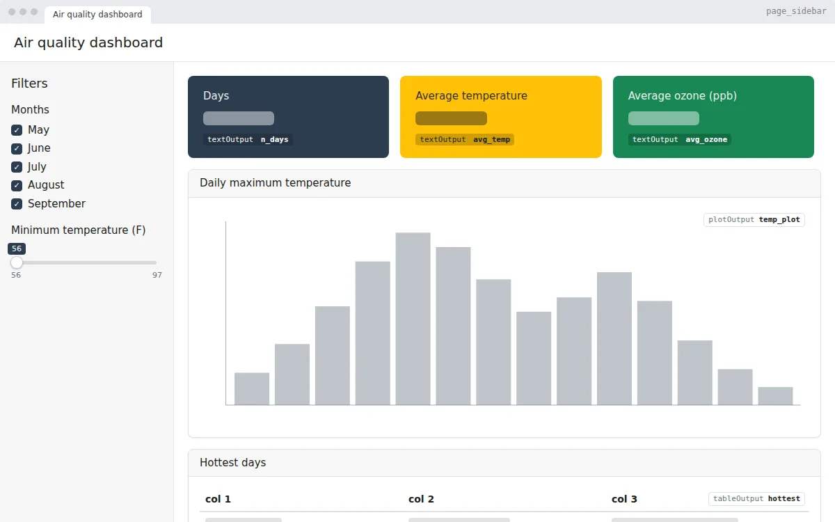
KPI dashboard
A Shiny dashboard with KPI value boxes, sidebar filters, a chart and a top-5 table, built with bslib on R’s airquality data. Free app.R to copy, edit and run.
The classic first Shiny app, rebuilt with bslib: a slider and a variable picker drive a histogram of the Old Faithful geyser data. Free app.R to copy and run.
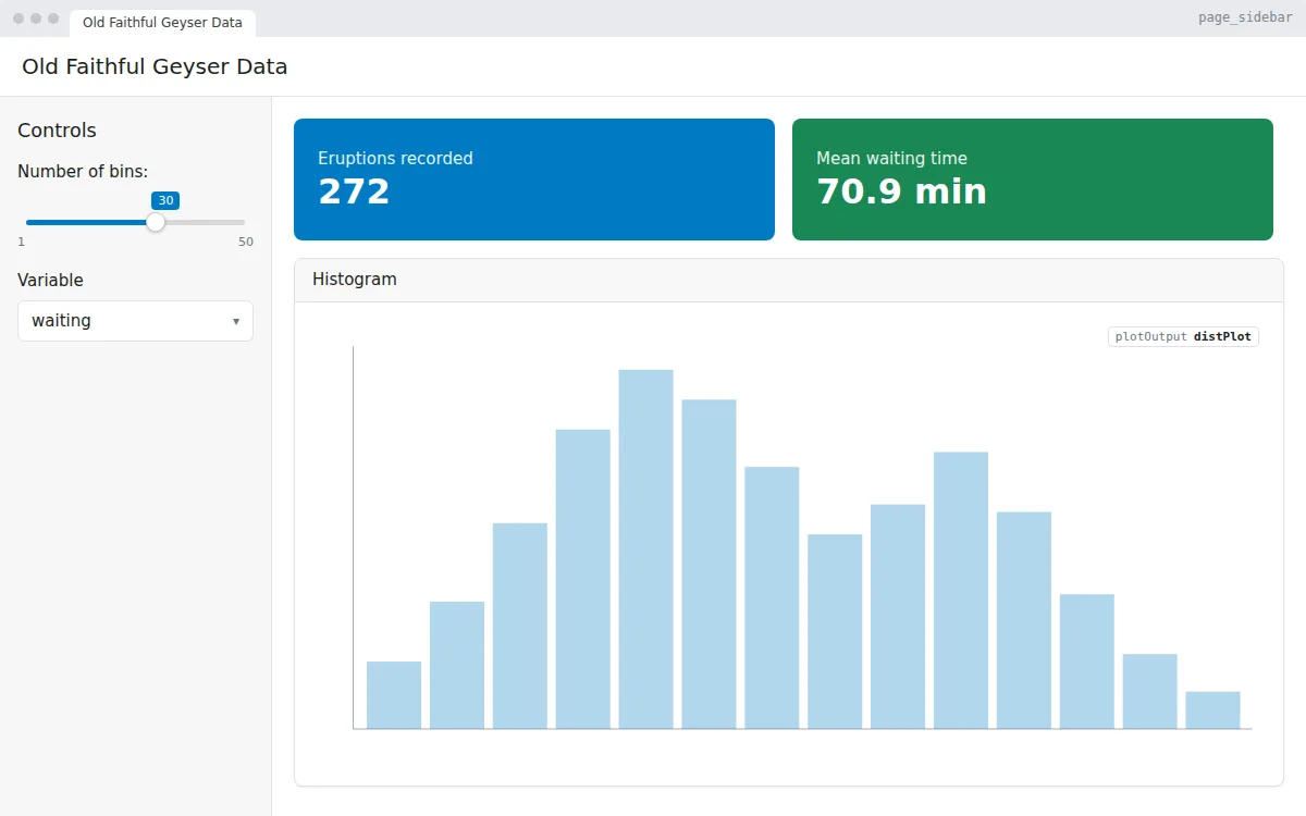
The app most people meet first when they learn Shiny, in a modern bslib layout. A slider sets the number of bins and a drop-down picks the variable, and the histogram redraws as you change them.
It is the smallest complete example of Shiny’s reactivity: two inputs, one output and a few lines of server code. A good template for a single chart with a couple of controls.
page_sidebar() layout with inputs in the sidebarsliderInput() and a selectInput()layout_columns() gridrenderPlot()# Generated by DropToApp
library(shiny)
library(bslib)
ui <- page_sidebar(
title = "Old Faithful Geyser Data",
sidebar = sidebar(
title = "Controls",
sliderInput("bins", "Number of bins:", min = 1, max = 50, value = 30),
selectInput(
"var",
"Variable",
choices = c("waiting", "eruptions"),
selected = "waiting"
)
),
layout_columns(
value_box(
title = "Eruptions recorded",
value = "272",
theme = "primary"
),
value_box(
title = "Mean waiting time",
value = "70.9 min",
theme = "success"
)
),
card(
full_screen = TRUE,
card_header("Histogram"),
plotOutput("distPlot")
)
)
server <- function(input, output, session) {
# Inputs: input$bins, input$var
output$distPlot <- renderPlot({
x <- faithful[[input$var]]
bins <- seq(min(x), max(x), length.out = input$bins + 1)
hist(x, breaks = bins, col = "#007bc2", border = "white",
xlab = input$var, main = NULL)
})
}
shinyApp(ui, server)
app.R, install the packages once with install.packages(c("shiny", "bslib")), then run shiny::runApp() in the folder with the file.app.R.
A Shiny dashboard with KPI value boxes, sidebar filters, a chart and a top-5 table, built with bslib on R’s airquality data. Free app.R to copy, edit and run.
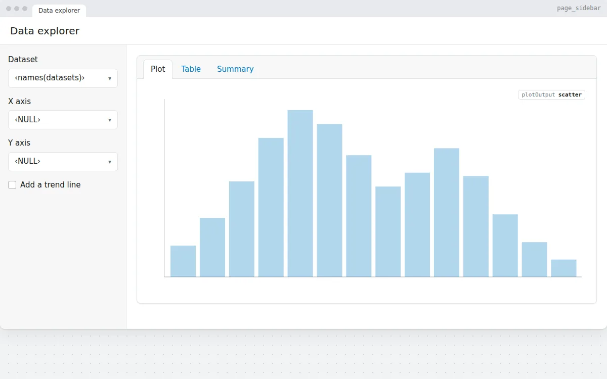
Pick a dataset and two columns to get a scatter plot, a searchable DT table and a summary, with axis choices that update per dataset. Free R Shiny template.
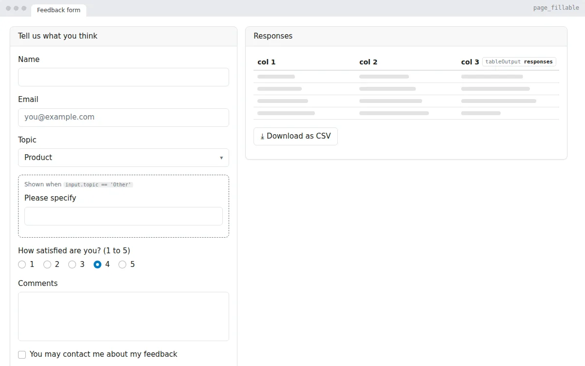
A feedback form in R Shiny: text, choice and rating inputs, a conditional field, validation, a live table of responses and a CSV download. Free app.R.
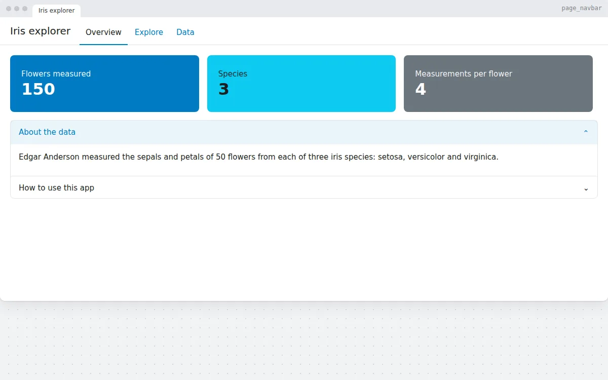
A Shiny app with several pages in a navigation bar: an overview with value boxes and an accordion, an interactive plotly chart and a DT data table.
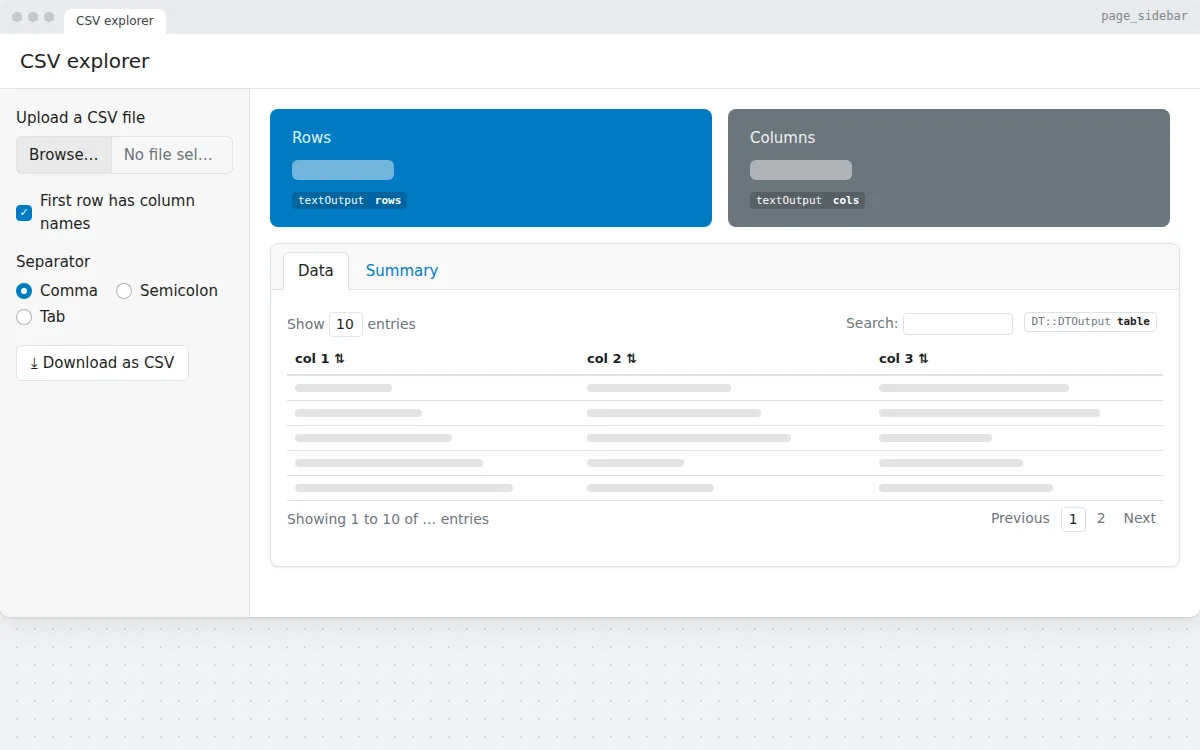
Upload a CSV file, choose the separator, and see its rows, columns, a searchable table and a summary. Download the data again as CSV. Free Shiny app template.